2 mm Scope Lens Distortion: Demand a Residual, Not a Promise

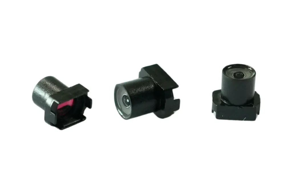
A 2 mm scope lens can be pushed to a few percent of distortion across the central field, but a perfectly flat, rectilinear margin at the extreme edge is not a realistic demand at this diameter. The honest requirement is a measured distortion map, a stated mapping convention, and a residual geometric error after calibration, quoted per annulus in object-space units. Ask the maker to prove the limit with a same-constraint comparison: the same design goal optimized again at 2.5 mm or 3.0 mm, or at a narrower field of view, plus unit-to-unit spread measured on production units. Without that comparison, the margin you were shown is a capability gap, not a physical wall.

If this matches an optic you are sourcing, the Lensmind endoscope lens family covers the standard diameters and FOV options we keep in production.

What a 2 mm diameter really constrains

The outer diameter is a packaging number, not an optical one. Once the barrel wall and the cover glass take their share, the active aperture of a 2 mm scope objective is a fraction of a millimetre, and the practical way to get a useful field of view through it is a wide-angle front group built with negative power. That negative front element is what bends the marginal rays hard, so barrel distortion at the margin follows from the design choice rather than from an assembly defect. Four things pull against each other in an envelope this small: field angle, aperture, edge resolution and package size on one side, low distortion and flat magnification on the other. A 2 mm build normally buys one or two of them properly. It also pays to separate straight-line rendering error from the defects software cannot repair, which is the distinction the standard description of optical distortion makes: field curvature, astigmatism, coma and steep-angle shading do not come back when you remap pixels.

Typical uncorrected distortion levels in 2 mm microendoscopes follow from that geometry. A few percent across the useful central field is a reasonable high-performance target, roughly 5 to 10 percent near the outer field is normal for a wide 2 mm class design, and 10 to 20 percent at the extreme edge is not by itself proof of poor manufacturing. Those figures describe the raw optic. The number that decides whether your software can work is what remains after correction, so treat the raw percentage as a description and the residual as a specification. It also helps to know which sensor the objective will feed, because the pixel grid sets the scale on which residual error is measured; the sensor pairing for sub-2 mm objectives is part of the distortion budget, not a separate purchase.

Choose the mapping before you choose the distortion number

The word flat hides a decision that changes the demand on the glass. A rectilinear mapping, also written f-tan theta, keeps straight lines straight and is what most measurement software assumes by default. An equidistant mapping, f-theta, puts equal angular steps at equal image steps, which is what a very wide front group tends to produce naturally. If your software can be told to unwrap the image with an equidistant model, the margin needs far less geometric stretching, and the residual after correction often drops without touching the lens. If the software insists on rectilinear output, that requirement belongs in the optical specification, because at 2 mm it is a real design demand rather than a formatting preference.

The second trap is the denominator. Percentage distortion means nothing until the reference is named: the same lens can be quoted as about 3 percent or about 12 percent depending on whether the divisor is the ideal image height, the object height, or the maximum field height. Distortion is properly established from paired object-side and image-side coordinates, so the convention belongs in the quotation. For anything dimensional, ask for the error in object-space units at your working distance, in millimetres or in micrometres, because that is the quantity your process can budget. The wider treatment of what a distortion figure covers and what it leaves out in an industrial setting is worth reading alongside this, in our note on what a distortion specification of 0.05 percent actually means.

The number that belongs in the drawing

Objective criteria for acceptable distortion in medical endoscopes and industrial scopes beat any adjective, and realistic optical distortion specifications for 2 mm lenses can be written as a single clause. It reads like this: over the stated working-distance range, at the specified focus and temperature, after the supplied calibration, the maximum residual geometric error shall not exceed X pixels or Y percent of the measured field height, whichever is smaller, with separate limits for the central part of the field and for the outer annulus, and with regions that fail the criterion explicitly masked and reported. Three details in that sentence carry most of the value. The per-annulus split stops one good central number from hiding a margin your software cannot use. The mask turns the usable field into a measured quantity rather than a claim, so nobody counts interpolated edge pixels as data. And the stated focus and temperature give the calibration a validity domain instead of leaving it as a one-time experiment. Quantifying optical distortion in 2 mm endoscopes is therefore a clause-writing exercise as much as a measurement one.

Add the sampling cost to the same clause. Rectification stretches pixels outward near the margin, so the effective resolution in the outermost annulus falls by roughly the local scale factor, and the valid measurement region shrinks at the same time. Ask the maker to state the usable image circle after rectification and the resolution you can expect inside it. Micro-endoscope image distortion correction rarely fails because the model is too simple; it fails because nobody fixed the reference before the lens was designed. An optical distortion tolerance for 2 mm endoscope lenses that ignores this will pass on paper and fail on the bench, because a geometrically straight edge with too few pixels across it is still a soft edge to a measuring algorithm.

What the maker must show to prove the limit

Measuring and proving optical distortion limits is a documentation exercise, so ask for measured data from a fabricated unit rather than a design plot. The package should open with raw frames of a precision grid or dot target that spans the full usable field, with the target’s flatness, pitch accuracy, working distance, focus setting, illumination and sensor stated. From those frames the maker should extract the measured coordinates of every target point, the fitted projection model, and the residual vector field that remains after the fit. Radial and tangential components should be reported separately, because a large tangential term points at centring and tilt rather than at the prescription, and no radial model will absorb it.

Two or three calibration models should be tried, for example a polynomial model and a dense lookup-table remap, and the comparison that matters is the maximum and RMS residual after correction, not the coefficient values. Image quality has to travel with the geometry: MTF or line-pair results at the centre, mid-field and edge, in both tangential and sagittal directions, plus the best-focus position per field location together with the depth of field at your working distance. The protocol should cover several production units rather than one laboratory sample, including lens reinstallation, orientation, and the spread across a batch. Manufacturer data for proving optical performance limits of micro-lenses is useful in that form: raw frames, target dimensions, calibration model, map or lookup table, valid region, interpolation method, and the tolerance attached to each number.

The comparison that answers the original question is a trade curve rather than a single result: distortion against field angle, distortion against usable field of view, edge MTF against distortion, and predicted performance for the current 2 mm package against 2.5 mm and 3.0 mm versions of the same goal, with Monte Carlo tolerance results behind the figures. That is the difference between a measured capability and a proven limit.

Where the manufacturing limit actually lives

At this diameter the prescription is rarely the binding constraint; the assembly is. Centring error and element tilt generate asymmetric distortion that shifts with unit, orientation and reinstallation, which is why batch spread rather than the nominal curve is where a program usually gets into trouble. Ask for the maker’s process data on centring and focus, not only a final field test, so that a drift at the margin surfaces before a shipment does.

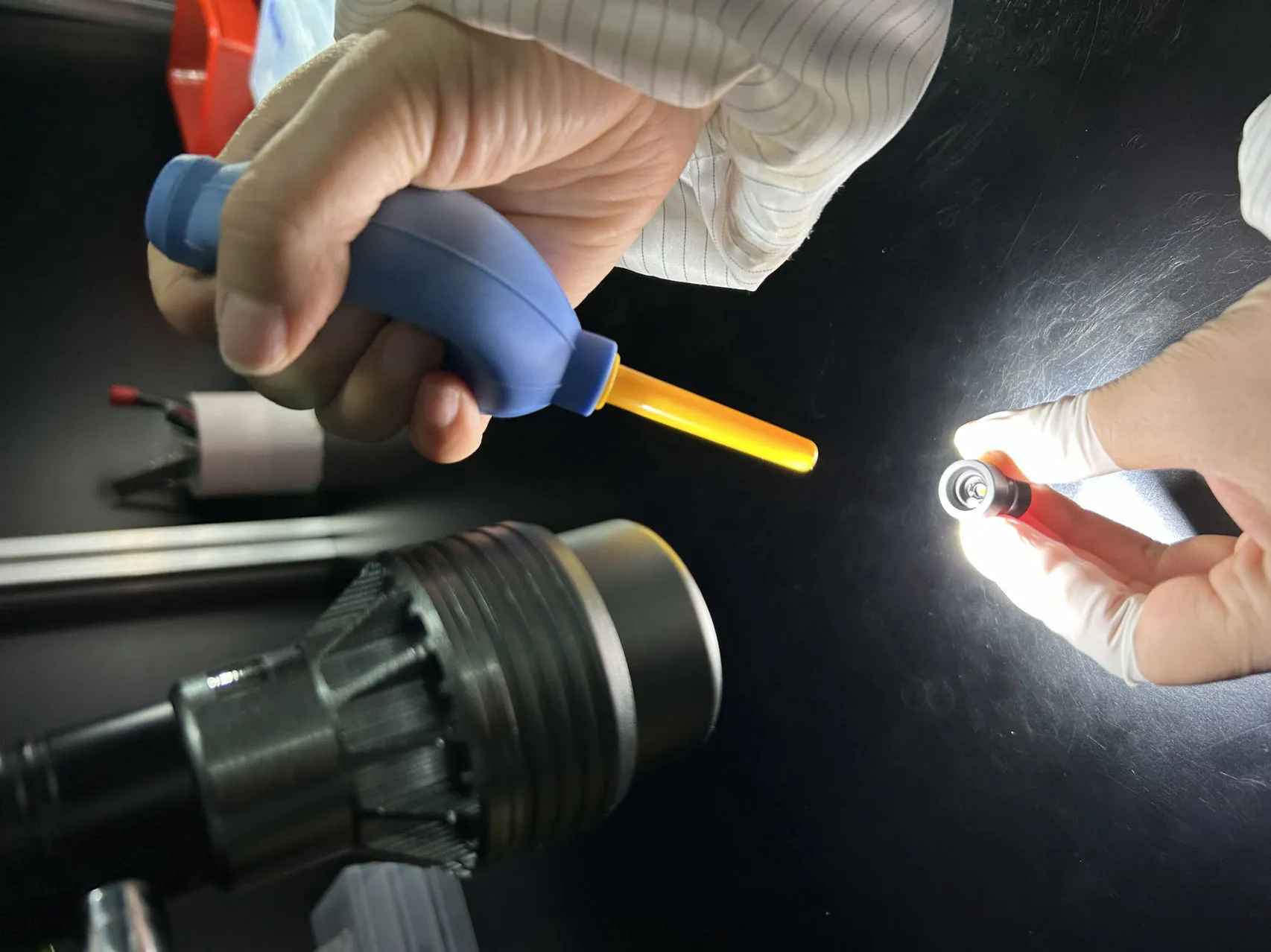
Lensmind builds endoscope and miniature objectives with in-house machining, cementing, cleanroom assembly and final metrology, in Class 10,000 (ISO Class 7 equivalent) cells zoned for medical and harsh-environment work, with 1 micrometre-class active alignment where a design needs it and measurement on systems that include Trioptics centring and OptiSurf instruments, a laser Fizeau interferometer, a UV spectrophotometer and reflective centring instruments. That equipment matters to this argument because centring data is the leading indicator of margin distortion, and a maker who can show it can also demonstrate unit-to-unit spread without running a special project. The manufacturing limits of micro-endoscope lenses show up first in centration numbers and last in a finished field test.

Sorting a real limit from a capability gap, then writing it into the RFQ

When a maker says flat geometry is impossible at 2 mm, the useful reply is a request for numbers: at which radius, at which field angle, at which working distance, with what residual error, and which mechanism sets the wall, whether that is distortion, field curvature, resolution, vignetting or tolerance. If the answer is that the design cannot be improved, the proof is a comparison of optimised designs under identical constraints, plus yield data showing what the current design delivers in production. This is also where standards vocabulary helps and where it needs care. The ISO 8600-5 endoscope testing procedure is an optical resolution method, so it will not settle a distortion argument; the distortion criteria have to live in your purchase specification, with ISO 9039 as the shared language for how the measurement itself is defined. Naming the standard you expect, and the number you expect against it, removes most of the room for interpretation later.

Then put the whole argument into the procurement documents. The RFQ should carry the residual clause, the evidence pack, the trade curve, and a first-article measurement against your own target frames. Documentation that ships with production should be named in advance: the agreed family parameters, typically MTF, distortion, BFL and DOF, with batch number, test conditions, inspection coverage and an explicit pass or fail judgment. That pack is the normal deliverable here rather than a special request, and it is the difference between buying a lens and renting a promise. For scale, the FA machine vision line holds distortion below 0.05 percent with 10K+ batch consistency, a figure that means something only because it is measured on the terms described above. Custom feasibility comes back within 48 hours, an NDA can be signed before drawings move, and prototype to mass production is a written 60 working day commitment.